Linear Regression Using Microsoft Excel

In this post, we will talk about the multiple linear regression using Excel. We will learn about the basic assumptions of classical linear regression model, performing regression using Excel, and interpreting the result.

Let’s start with the basic definition of regression analysis.

The term regression was introduced by Francis Galton in their research paper. Modern interpretation of Regression analysis is concerned with the study of dependence of one variable (dependent variable), on one or more other variables (the explanatory or independent variables), with a view of estimating or predicting the dependent variable’s value in terms of independent variables.

Method of estimation:

There are two mostly used method of estimation

      1-      Ordinary Least Squares (OLS)

      2-      Maximum Likelihood (ML)

OLS is highly used method for estimation because it is intuitive appealing and simpler than ML method. Besides, in linear regression context the both methods generally give similar results.

Assumptions of OLS method:

These are the following assumptions of OLS. Under these assumptions, OLS has some useful statistical properties which makes it one of the most powerful method of regression analysis. Regression model will be valid under the following assumptions.

1-      Regression model is linear in parameters, though it may or may not be linear in the variables i.e. regressand Y and regressor X may be nonlinear.

                                                         Y_i = β₀ + β₁ X_i + u_i

2-      Fixed regressor X or X values are independent of the error term

                                                  i.e. covariance(X_{i ,}u_i) = 0

3-      Expected value or mean of error term (random disturbance) is zero.

                                                                E(u_i) = 0

4-      Variance of error term (random disturbance) is same regardless of the value of regressor X. This property is called Homoscedasticity (Home – equal , Scedasticity – spread i.e. equal variance)

                                                             Var(u_i) = σ²

               Homoscedasticity refers to the assumption that that the dependent variable exhibits similar   amounts of variance across the range of values for an independent variable.

                                             

               Heteroscedasticity is the absence of homoscedasticity.

5-      No Autocorrelation between the any 2 error terms (random disturbances).

                                                  covariance(u_{i ,}u_j) = 0             i ≠ j

6-      No Multicollinearity between the any 2 regressors or X values.

                                                  covariance(X_{i ,}X_j) = 0             i ≠ j

7-      Number of observations must be greater than number of parameters to be estimated.

                                              

For example, we have the data set for a store who sells cold drinks. We need to find out the relation between the demand of cold drink (dependent variable) and the price of cold drink & advertisement expenses done (independent variable).

Week	Demand (Q)	Price (P)	Ad Expenses (A)
1	51345	2.78	4280
2	50337	2.35	3875
3	86732	3.22	12360
4	118117	1.85	19250
5	48024	2.65	6450
6	97375	2.95	8750
7	75751	2.86	9600
8	78797	3.35	9600
9	59856	3.45	9600
10	23696	3.25	6250
11	61385	3.21	4780
12	63750	3.02	6770
13	60996	3.16	6325
14	84276	2.95	9655
15	54222	2.65	10450
16	58131	3.24	9750
17	55398	3.55	11500
18	69943	3.75	8975
19	79785	3.85	8975
20	38892	3.76	6755
21	43240	3.65	5500
22	52078	3.58	4365
23	11321	3.78	9525
24	73113	3.75	18600
25	79988	3.22	14450
26	98311	3.42	15500
27	78953	2.27	21225
28	52875	3.78	7580
29	81263	3.95	4175
30	67260	3.52	4365
31	83323	3.45	12250
32	68322	3.92	11850
33	71925	4.05	14360
34	29372	4.01	9540
35	21710	3.68	7250
36	37833	3.62	4280
37	41154	3.57	13800
38	50925	3.65	15300
39	57657	3.89	5250
40	52036	3.86	7650
41	58677	3.95	6650
42	73902	3.91	9850
43	55327	3.88	8350
44	16262	4.12	10250
45	38348	3.94	16450
46	29810	4.15	13200
47	69613	4.12	14600
48	45822	4.16	13250
49	43207	4	18450
50	81998	3.93	16500
51	46756	3.89	6500
52	34593	3.83	5650

Performing multiple regression in Excel

      1-      Click on the data tab. Then click on the menu Data Analysis at the corner. Then a pop up window will open. Now select Regression from this pop up window. And click in OK.

       2-      Now a pop up window will open asking for inputs. Now click on arrow sign to select the X range (Regressor) and Y range.

 

      3-      You can select any of the parameters like confidence interval (by default it is 95%) or any other as per your requirement.

      4-      Now select the output range. You have options to get output in same work sheet, new worksheet and new workbook. Here we want to get output in same worksheet and selected a range. As you can see in above pic. Now press OK to get output.

 

Interpretation of regression output:

Regression Statistics table:

Multiple R – is the coefficient of multiple correlation. You may be knowing the bivariate correlation. Multiple correlation can be interpreted in the same way. R is a measure of the strength of the association between the independent variables and the one dependent variable.

                                              

R Square – is the square of Multiple R. It is called as multiple coefficient of determination. It is useful to explain that how much of total variation can be explained by the predicted model. It is measure of goodness of fit of predicted model.

In our case R square = 0.263782. It means that 26.37% of the variation (variation of Y around its mean) can be explained by the model (by independent variables).

Unfortunately, in case of multiple regression R square is not the unbiased estimation of coefficient of determination. Adjusted R square is a better estimate for coefficient of determination in case of multiple regression.

Adjusted R Square - It indicates that how much of total variation can be explained by the model, adjusted for the degree of freedom. It should be used in place of R square for multiple regression

                                                     

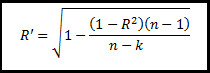
Where k = the number of variables in the model (Independent as well as dependent)  and n = the number of data elements in the sample.

In our case, k=3 (2 IV, and 1DV) , and n =52

Standard Error - refers to the estimated standard deviation of the error term u. Sometimes it is called as standard error of the regression.

                                                  Standard Error = sqrt(Square sum of error ∕(n-k))

ANOVA Table:

Sum Squares (SS) corresponding to regression is called Explained Sum Square (ESS) or Sum Square Regression (SSR).

Sum Squares (SS) corresponding to residual is called Residual Sum Square (RSS) or Sum Square Error (SSE).

Total Sum Square (TSS) = ESS + RSS

Mean Sum Square = SS/df

Significance of F – indicates weather value of R square is significant or not i.e. significance of measure of goodness of fit.

Coefficients - gives the least squares estimates of β_j.

Standard error- gives the standard errors of the least squares estimates b_j of β_j.

t Stat-  gives the computed t-statistic for hypotheses H0: β_j = 0 against Ha: β_j ≠ 0. It checks for the significance of the parameter β_j values. Also called as significance test.

T stat = Coefficients / Standard error. It is compared to a t value from t-table with df degrees of freedom and a particular confidence interval (1-α).

P-value- gives the p-value for test of H0: β_j = 0 against Ha: β_j ≠ 0. It is the testing of hypotheses.

As we have taken a confidence interval of 95%. So, if p-value corresponding to a parameter is less than 0.05. Then, we will reject the Null Hypothesis i.e. β_j ≠ 0 or is significant.

Note that this p-value is for a two-sided test. For a one-sided test divide this p-value by 2 (also checking the sign of the t-Stat).

Columns Lower 95% and Upper 95% values define a 95% confidence interval for β_j.

Estimated Regression Model:

Estimated Industry Demand (Q cap) = 100626.034 -16392.63 * Price (P) + 1.5763295 * Ad Expense (A)