Analytics For Business

Monday 19 October 2015

Choosing a Rotation Method for Factor analysis in SPSS

In this post, we will discuss about the different rotation methods available in SPSS, and use each of method.

We will start with the definition of rotation and usefulness of rotation in factor and principal component analysis.

According to Yaremko, Harari, Harrison, and Lynn, factor rotation is as follows:
“In factor or principal-components analysis, rotation of the factor axes (dimensions) identified in the initial extraction of factors, in order to obtain simple and interpretable factors.”


Types of Rotation:  There are 2 types of rotations.
      1-      Orthogonal Rotation: These methods assumes that the factors or components in analysis are uncorrelated.
a.       Varimax Method: minimizes the number of variables that have high loadings on each factor. This method simplifies the interpretation of the factors.
b.      Quartimax Method: minimizes the number of factors needed to explain each variable. This method simplifies the interpretation of the observed variables.
c.       Equamax Method: combination of the varimax method, which simplifies the factors, and the quartimax method, which simplifies the variables. The number of variables that load highly on a factor and the number of factors needed to explain a variable are minimized.

      2-      Oblique Rotation: SPSS has two oblique rotation methods.
a.       Direct oblimin Method
b.      Promax Method: can be calculated more quickly than a direct oblimin rotation, so it is useful for large datasets.

Decision to choose a rotation method:
Tabachnick and Fiddell argue that “Perhaps the best way to decide between orthogonal and oblique rotation is to request oblique rotation [e.g., direct oblimin or promax from SPSS] with the desired number of factors and look at the correlations among factor. If factor correlations are not driven by the data, the solution remains nearly orthogonal. Look at the factor correlation matrix for correlations around .32 and above. If correlations exceed .32, then there is 10% (or more) overlap in variance among factors, enough variance to warrant oblique rotation unless there are compelling reasons for orthogonal rotation.”

Moreover, as Kim and Mueller put it, “Even the issue of whether factors are correlated or not may not make much difference in the exploratory stages of analysis. It even can be argued that employing a method of orthogonal rotation (or maintaining the arbitrary imposition that the factors remain orthogonal) may be preferred over oblique rotation, if for no other reason than that the former is much simpler to understand and interpret.”

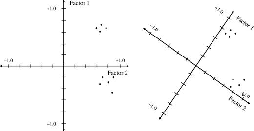
We can think of the goal of rotation and of choosing a particular type of rotation as seeking something called simple structure.

Bryant and Yarnold define simple structure as:
A condition in which variables load at near 1 (in absolute value) or at near 0 on an eigenvector (factor). Variables that load near 1 are clearly important in the interpretation of the factor, and variables that load near 0 are clearly unimportant. Simple structure thus simplifies the task of interpreting the factors.

Thurstone’s 5 criteria to choose a rotation method:
Thurstone first proposed and argued for five criteria that needed to be met for simple structure to be achieved:
      1-      Each variable should produce at least one zero loading on some factor.
      2-       Each factor should have at least as many zero loadings as there are factors.
      3-      Each pair of factors should have variables with significant loadings on one and zero loadings on the other.
      4-      Each pair of factors should have a large proportion of zero loadings on both factors (if there are say four or more factors total).
      5-      Each pair of factors should have only a few complex variables.

Zero loading- One rule of thumb is that zero loadings includes any that fall between -.10 and +.10.

Significant loading- With a sample size of say 100 participants, loadings of .30 or higher can be considered significant, or at least salient. With much larger samples, even smaller loadings could be considered salient, but in language research, researchers typically take note of loadings of .30 or higher.

Complex variables- Variables with loadings of .30 or higher on more than one factor


Sunday 18 October 2015

Linear Regression Using Microsoft Excel


In this post, we will talk about the multiple linear regression using Excel. We will learn about the basic assumptions of classical linear regression model, performing regression using Excel, and interpreting the result.
Let’s start with the basic definition of regression analysis.
The term regression was introduced by Francis Galton in their research paper. Modern interpretation of Regression analysis is concerned with the study of dependence of one variable (dependent variable), on one or more other variables (the explanatory or independent variables), with a view of estimating or predicting the dependent variable’s value in terms of independent variables.
Method of estimation:
There are two mostly used method of estimation
      1-      Ordinary Least Squares (OLS)
      2-      Maximum Likelihood (ML)
OLS is highly used method for estimation because it is intuitive appealing and simpler than ML method. Besides, in linear regression context the both methods generally give similar results.
Assumptions of OLS method:
These are the following assumptions of OLS. Under these assumptions, OLS has some useful statistical properties which makes it one of the most powerful method of regression analysis. Regression model will be valid under the following assumptions.
1-      Regression model is linear in parameters, though it may or may not be linear in the variables i.e. regressand Y and regressor X may be nonlinear.
                                                         Yi = β0 + β1 Xi + ui
2-      Fixed regressor X or X values are independent of the error term
                                                  i.e. covariance(Xi ,ui) = 0
3-      Expected value or mean of error term (random disturbance) is zero.
                                                                E(ui) = 0
4-      Variance of error term (random disturbance) is same regardless of the value of regressor X. This property is called Homoscedasticity (Home – equal , Scedasticity – spread i.e. equal variance)
                                                             Var(ui) = σ2
               Homoscedasticity refers to the assumption that that the dependent variable exhibits similar   amounts of variance across the range of values for an independent variable.
                                             

               Heteroscedasticity is the absence of homoscedasticity.
5-      No Autocorrelation between the any 2 error terms (random disturbances).
                                                  covariance(ui ,uj) = 0             i ≠ j
6-      No Multicollinearity between the any 2 regressors or X values.
                                                  covariance(Xi ,Xj) = 0             i ≠ j
7-      Number of observations must be greater than number of parameters to be estimated.
                                              
For example, we have the data set for a store who sells cold drinks. We need to find out the relation between the demand of cold drink (dependent variable) and the price of cold drink & advertisement expenses done (independent variable).
Week
Demand (Q)
Price (P)
Ad Expenses (A)
1
51345
2.78
4280
2
50337
2.35
3875
3
86732
3.22
12360
4
118117
1.85
19250
5
48024
2.65
6450
6
97375
2.95
8750
7
75751
2.86
9600
 8
78797
3.35
9600
9
59856
3.45
9600
10
23696
3.25
6250
11
61385
3.21
4780
12
63750
3.02
6770
13
60996
3.16
6325
14
84276
2.95
9655
15
54222
2.65
10450
16
58131
3.24
9750
17
55398
3.55
11500
18
69943
3.75
8975
19
79785
3.85
8975
20
38892
3.76
6755
21
43240
3.65
5500
22
52078
3.58
4365
23
11321
3.78
9525
24
73113
3.75
18600
25
79988
3.22
14450
26
98311
3.42
15500
27
78953
2.27
21225
28
52875
3.78
7580
29
81263
3.95
4175
30
67260
3.52
4365
31
83323
3.45
12250
32
68322
3.92
11850
33
71925
4.05
14360
34
29372
4.01
9540
35
21710
3.68
7250
36
37833
3.62
4280
37
41154
3.57
13800
38
50925
3.65
15300
39
57657
3.89
5250
40
52036
3.86
7650
41
58677
3.95
6650
42
73902
3.91
9850
43
55327
3.88
8350
44
16262
4.12
10250
45
38348
3.94
16450
46
29810
4.15
13200
47
69613
4.12
14600
48
45822
4.16
13250
49
43207
4
18450
50
81998
3.93
16500
51
46756
3.89
6500
52
34593
3.83
5650


Performing multiple regression in Excel
      1-      Click on the data tab. Then click on the menu Data Analysis at the corner. Then a pop up window will open. Now select Regression from this pop up window. And click in OK.

       2-      Now a pop up window will open asking for inputs. Now click on arrow sign to select the X range (Regressor) and Y range.


      3-      You can select any of the parameters like confidence interval (by default it is 95%) or any other as per your requirement.


      4-      Now select the output range. You have options to get output in same work sheet, new worksheet and new workbook. Here we want to get output in same worksheet and selected a range. As you can see in above pic. Now press OK to get output.

 
Interpretation of regression output:
Regression Statistics table:
Multiple R – is the coefficient of multiple correlation. You may be knowing the bivariate correlation. Multiple correlation can be interpreted in the same way. R is a measure of the strength of the association between the independent variables and the one dependent variable.
                                              

R Square – is the square of Multiple R. It is called as multiple coefficient of determination. It is useful to explain that how much of total variation can be explained by the predicted model. It is measure of goodness of fit of predicted model.
In our case R square = 0.263782. It means that 26.37% of the variation (variation of Y around its mean) can be explained by the model (by independent variables).
Unfortunately, in case of multiple regression R square is not the unbiased estimation of coefficient of determination. Adjusted R square is a better estimate for coefficient of determination in case of multiple regression.
Adjusted R Square - It indicates that how much of total variation can be explained by the model, adjusted for the degree of freedom. It should be used in place of R square for multiple regression
                                                     

Where k = the number of variables in the model (Independent as well as dependent)  and n = the number of data elements in the sample.
In our case, k=3 (2 IV, and 1DV) , and n =52
Standard Error - refers to the estimated standard deviation of the error term u. Sometimes it is called as standard error of the regression.
                                                  Standard Error = sqrt(Square sum of error ∕(n-k))

ANOVA Table:
Sum Squares (SS) corresponding to regression is called Explained Sum Square (ESS) or Sum Square Regression (SSR).
Sum Squares (SS) corresponding to residual is called Residual Sum Square (RSS) or Sum Square Error (SSE).
Total Sum Square (TSS) = ESS + RSS
Mean Sum Square = SS/df
Significance of F – indicates weather value of R square is significant or not i.e. significance of measure of goodness of fit.


Coefficients - gives the least squares estimates of βj.
Standard error- gives the standard errors of the least squares estimates bj of βj.
t Stat-  gives the computed t-statistic for hypotheses H0: βj = 0 against Ha: βj ≠ 0. It checks for the significance of the parameter βj values. Also called as significance test.
T stat = Coefficients / Standard error. It is compared to a t value from t-table with df degrees of freedom and a particular confidence interval (1-α).
P-value- gives the p-value for test of H0: βj = 0 against Ha: βj ≠ 0. It is the testing of hypotheses.
As we have taken a confidence interval of 95%. So, if p-value corresponding to a parameter is less than 0.05. Then, we will reject the Null Hypothesis i.e. βj ≠ 0 or is significant.
Note that this p-value is for a two-sided test. For a one-sided test divide this p-value by 2 (also checking the sign of the t-Stat).
Columns Lower 95% and Upper 95% values define a 95% confidence interval for βj.

Estimated Regression Model:

Estimated Industry Demand (Q cap) = 100626.034 -16392.63 * Price (P) + 1.5763295 * Ad Expense (A)